URL
TL;DR
- 这篇论文首次提出了
Denoising Diffusion Probabilistic Models (DDPM) 模型,该模型是一种去噪扩散模型,可以用于生成图像。
DDPM 有详细的热力学理论基础(Langevin 朗之万动力学),对热力学扩散过程进行了建模。- 本质上,
DDPM 是一个自回归生成模型,通过自监督方式,对图像进行添加噪声和逐步去噪的过程,来学习图像的分布。
Algorithm
DDPM 总体结构
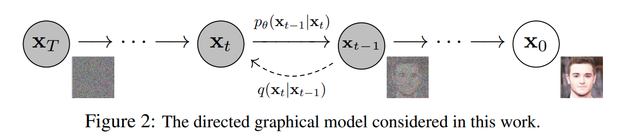
- 上图中 x0 是来自图像数据集的真实图像,从右到左被称为前向过程,即对图像逐步添加随机高斯噪声,直到得到噪声图像 xT
- 从左到右被称为逆向过程,即模型预测噪声,代入公式逐步去噪
前向过程
xt=1−βt⋅xt−1+βt⋅ϵt−1 , ϵt−1∼N(0,I)
- 其中:
- ϵt 是随机高斯噪声,即
torch.randn
- βt 是超参数,控制噪声的强度,随着 t 的增大,βt 从
1e-4 逐渐增大到 2e-2
- 总时间步数 T=1000
前向过程的累积表示
xt=αˉt⋅x0+1−αˉt⋅ϵ
- 具体推理过程:
- x1=1−β1⋅x0+β1⋅ϵ0
- x2=1−β2⋅x1+β2⋅ϵ1
- 将 x1 代入 x2 的公式中,得到 x2 的累积表示: x2=1−β2⋅(1−β1⋅x0+β1⋅ϵ0)+β2⋅ϵ1
- x2=1−β21−β1x0+1−β2β1⋅ϵ0+β2⋅ϵ1
- 以此类推,得到 xt 的累积表示:xt=∏i=1t(1−βi)⋅x0+∑i=1t∏j=i+1t(1−βj)⋅βi⋅ϵ
- 令 αˉt=∏i=1t(1−βi),得到 xt=αˉt⋅x0+∑i=1tβi⋅∏j=i+1t(1−βj)⋅ϵ
- 需要将噪声项合并成一个正态分布,需要确定方差,对于每一项 βi⋅∏j=i+1t(1−βj),其方差为 βi⋅∏j=i+1t(1−βj)
- 总噪声的方差为 ∑i=1tβi⋅∏j=i+1t(1−βj)
- 代入 αˉt 到噪声项的方差中,得到总噪声的方差为 ∑i=1tβi⋅αˉiαˉt=αˉt⋅∑i=1tαˉiβi
- 由于 αˉiβi=αˉi1−αi=αˉi1−αˉi−11,因此使用 裂项求和 公式可得:∑i=1tαˉiβi=αˉt1−αˉ01
- 由于 αˉ0=1,因此 ∑i=1tαˉiβi=αˉt1−1
- 代入噪声总方差公式中,得到总噪声的方差为 αˉt⋅(αˉt1−1)=1−αˉt
- 因此,累加形式的前向过程可表示为:xt=αˉt⋅x0+1−αˉt⋅ϵ
- 累积表示的好处:
- 在给定 t 时,可以直接从 x0 生成 xt,而不需要逐步生成
- 通过单步表示到累积表示的数学推导过程,可以更好地理解噪声的累积方差
逆向过程
xt−1=αt1(xt−1−αˉtβt⋅ϵθ(xt,t))
- 其中:
- ϵθ(xt,t) 是模型预测的噪声,即
model(x_t, t)
- αt=1−βt
- αˉt=∏s=1tαs
- 由上述公式可知:预测得到的噪声并不会直接叠加到噪声图像上,而是利用扩散原理,根据噪声添加相关的超参数进行去噪
- 由于 ϵθ(xt,t) 是模型对于 xt 的预测,且 xt 也和模型预测有关,因此逆向过程是个数据依赖的过程,因此逆向过程的累积表示没有意义
训练过程
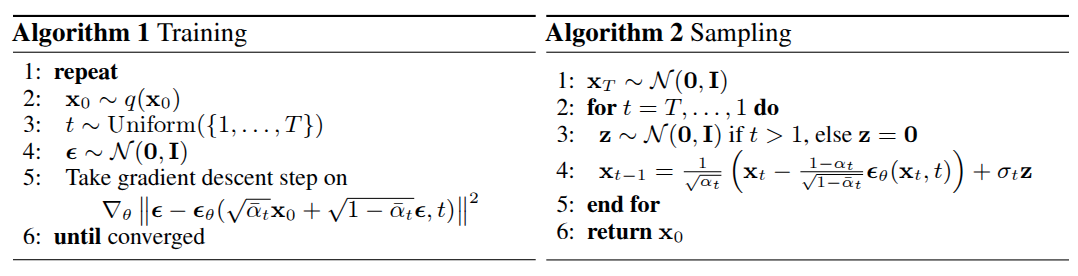
DDPM 的训练过程基于扩散模型的前向过程和逆向过程。训练的目标是让模型学习如何从噪声数据中恢复出原始数据。具体步骤如下:
- 输入数据:从数据集中随机选择一批原始图像 x0
- 随机选择扩散步数:对于每张图像,随机选择一个扩散步数 t,范围从 1 到 T 随机选择
- 生成噪声数据:通过前向过程生成噪声图像 xt
- 预测噪声:使用模型 ϵθ(xt,t) 预测添加到 x0 中的噪声
- 计算损失:通过比较预测噪声和真实噪声计算损失函数(通常是均方误差,
MSE)
- 更新模型参数:通过反向传播更新模型参数
伪代码
1
2
3
4
5
6
7
| for epoch in range(num_epochs):
for x0 in data_loader:
t = random.randint(1, T)
xt, noise = forward_diffusion(x0, t)
predicted_noise = model(xt, t)
loss = mse_loss(predicted_noise, noise)
update_model_parameters(loss)
|
模型输入输出
- 输入
- 原始图像 x0,通常被归一化到 [−1,1] 之间
- 扩散步数 t,随机选择,会变成
time embedding 输入模型
- 输出
- 预测噪声 ϵθ(xt,t),模型输出是预测的噪声,用于逆向过程去噪
损失函数
L(θ)=Ex0,t[∥ϵθ(xt,t)−ϵ∥2]
- 其中:
- ϵ 是真实噪声
- ϵθ(xt,t) 是模型预测的噪声
- Ex0,t 表示对所有的 x0 和 t 求期望
推理过程(采样过程)
用 pre-trained diffusion model 生成图像
1
2
3
4
5
6
7
8
9
10
11
12
13
14
15
16
17
18
19
20
21
22
23
24
25
26
27
28
29
30
31
32
33
34
| from diffusers import UNet2DModel
from diffusers import DDPMScheduler
from PIL import Image
import numpy as np
import tqdm
import torch
device = torch.device("cuda" if torch.cuda.is_available() else "cpu")
def display_sample(sample, i):
image_processed = sample.cpu().permute(0, 2, 3, 1)
image_processed = (image_processed + 1.0) * 127.5
image_processed = image_processed.numpy().astype(np.uint8)
image_pil = Image.fromarray(image_processed[0])
image_pil.save(f"sample_{i}.png")
repo_id = "google/ddpm-church-256"
model = UNet2DModel.from_pretrained(repo_id).to(device)
scheduler = DDPMScheduler.from_config(repo_id)
noisy_sample = torch.randn(
1, model.config.in_channels, model.config.sample_size, model.config.sample_size
)
sample = noisy_sample.to(device)
for i, t in enumerate(tqdm.tqdm(scheduler.timesteps)):
with torch.no_grad():
residual = model(sample, t).sample
sample = (
sample - (1 - alphas[t]) / torch.sqrt(1 - alphas_cumprod[t]) * residual
) / torch.sqrt(alphas[t])
if t > 1:
noise = torch.randn_like(sample).to(device)
sample += torch.sqrt(1 - alphas[t]) * noise
if (i + 1) % 50 == 0:
display_sample(sample, i + 1)
|
- 通过
UNet2DModel 加载预训练模型
- 通过
DDPMScheduler 构建调度器(主要作用是生成噪声和去噪)
- 通过
torch.randn 生成随机噪声作为输入
- 通过
scheduler.step 逐步生成图像
- 最终生成一张完全去噪的新图像,这张图像并不在任何数据集中(只是风格看起来像
Church-256 数据集),是模型自己生成的(这也意味着没办法去指导模型生成特定的图像)
用 pre-trained diffusion model 对已逐步添加噪声的图像去噪
- 理论上,可以将一张数据集中的图像逐步添加噪声,在 t=T 步之后,使用模型去噪,得到一张和原始图像非常相似的图像
- 但实际测试中,当 t 较大时(大于
300,T 等于 1000),得到的去噪图像和原始图像相差较大,在 t<300 时,去噪图像和原始图像相似度较高
1
2
3
4
5
6
7
8
9
10
11
12
13
14
15
16
17
18
19
20
21
22
23
24
25
26
27
28
29
30
31
32
33
34
35
36
37
38
39
40
41
42
43
44
45
46
47
48
49
50
| from diffusers import UNet2DModel
from diffusers import DDPMScheduler
from diffusers import DDPMPipeline
from PIL import Image
import numpy as np
import tqdm
import torch
device = torch.device("cuda" if torch.cuda.is_available() else "cpu")
def preprocess_image(image):
"""Preprocess an image to model input format."""
image = np.array(image).astype(np.float32) / 127.5 - 1.0
image = (
torch.tensor(image).permute(2, 0, 1).unsqueeze(0).to(device)
)
return image
def display_sample(sample, name):
"""Save a sample as an image."""
image_processed = sample.cpu().permute(0, 2, 3, 1)
image_processed = (image_processed + 1.0) * 127.5
image_processed = image_processed.numpy().astype(np.uint8)
image_pil = Image.fromarray(image_processed[0])
image_pil.save(f"{name}.png")
repo_id = "google/ddpm-celebahq-256"
image_pipe = DDPMPipeline.from_pretrained(repo_id).to(device)
image = image_pipe().images[0]
image.save("original_image.png")
original_image = preprocess_image(image)
model = UNet2DModel.from_pretrained(repo_id).to(device)
scheduler = DDPMScheduler.from_config(repo_id)
T = scheduler.num_train_timesteps
alpha_cumprod = scheduler.alphas_cumprod[300]
noisy_image = torch.sqrt(alpha_cumprod) * original_image + torch.sqrt(
1 - alpha_cumprod
) * torch.randn_like(original_image)
display_sample(noisy_image, "noisy_image")
sample = noisy_image.clone()
for t in tqdm.tqdm(scheduler.timesteps[-300:]):
with torch.no_grad():
residual = model(sample, t).sample
sample = (
sample - (1 - alphas[t]) / torch.sqrt(1 - alphas_cumprod[t]) * residual
) / torch.sqrt(alphas[t])
if t > 1:
noise = torch.randn_like(sample).to(device)
sample += torch.sqrt(1 - alphas[t]) * noise
display_sample(sample, "final_image")
l2_diff = torch.norm(original_image - sample).item()
print(f"L2 difference between original and final image: {l2_diff}")
|
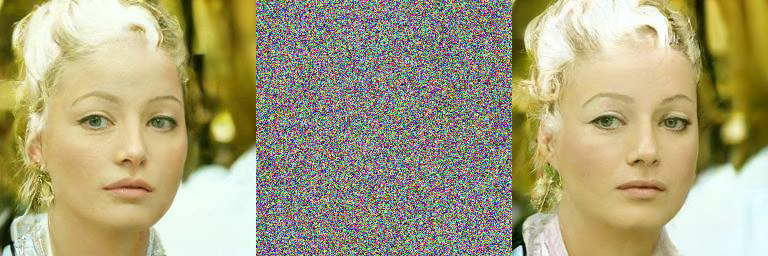
上图表示 t=300 时,原图 -> 噪声图 -> 去噪图

上图表示 t=500 时,原图 -> 噪声图 -> 去噪图

上图表示 t=1000 时,原图 -> 噪声图 -> 去噪图
Thoughts
DDPM 是一种非常有趣的生成模型,数学基础非常扎实- 但仍然存储三个主要问题:
- 时间步 T 太大,通常是
1000
- 无法指定模型生成特定的图像,只能生成和数据集相似的图像
- 作用在图像域,计算量较大
- 针对以上三个问题,
stable diffusion 诞生了