URL
- paper: https://arxiv.org/pdf/2506.21619
- code: https://github.com/index-tts/index-tts
- demo: https://index-tts.github.io/index-tts2.github.io
TL;DR
IndexTTS2是BiliBili提出的一种TTS模型,有如下几个特点:- 情感表达:能够生成具有特定情感的语音,如快乐、悲伤、愤怒等。
- 时长控制:可以通过输入一个数字来精确控制生成语音的时长。
- 零样本学习:无需针对特定说话人进行训练,能够适应新的说话人(常见的
TTS只提供少量的说话人音色供选择,IndexTTS2可以适配任何给定样本的音色)。 - 自回归生成:通过逐步生成语音帧,提升了语音的自然度和连贯性。
IndexTTS2的输入:- 源文本 (
Source Text):需要转换为语音的文字。 - 音色提示 (
Timbre Prompt):一小段目标说话人的音频,用于提取“音色”特征,决定了合成语音“像谁”。 - 风格提示 (
Style Prompt):一小段带有特定情感的音频,用于提取“情感”特征,决定了合成语音的“情绪”。 - 语音 Token 数量 (
Speech Token Num)(可选):一个数字,用于精确控制生成语音的时长。
- 源文本 (
IndexTTS2的输出:目标语音 (Target Speech):最终合成的音频波形文件。
Algorithm
0. 基础知识
0.1 语音的表示方法
- 连续表示:声音的物理基础
- 数字波形:数字波形(
Digital Waveform)是语音最直接、最基础的表示形式。它是通过对连续的模拟声波进行“采样”(Sampling)得到的。采样过程以固定的时间间隔(由采样率决定,如16000 Hz或24000 Hz)测量声波的振幅,从而将连续的信号转换为一个离散的数值序列。这个序列在时间维度上描绘了声音振幅的变化,因此也被称为声音的时域(time domain)表示。 - 梅尔频谱图:为了解决波形表示的难题,研究者们借鉴了人类听觉系统的特性,提出了一种更高效、更符合感知的表示方法——梅尔频谱图(
Mel-Spectrogram)。它是一种时频(time-frequency)表示,描绘了语音信号的能量如何随时间和频率变化。其生成过程大致如下:- 分帧与加窗:将长段的音频波形切分成许多短暂的、有重叠的“帧”(
frame),并对每一帧应用一个窗函数。 - 傅里叶变换:对每一帧进行短时傅里叶变换(
STFT),得到其频谱,即能量在不同频率上的分布。 - 梅尔尺度映射:将频谱的频率轴从线性的赫兹(
Hz)尺度,映射到梅尔(Mel)尺度。梅尔尺度是一种非线性尺度,它模拟了人耳对频率的感知特性——人耳对低频声音的变化比对高频声音的变化更敏感。 - 能量取对数:最后,通常会对能量值取对数,使其更符合人类对音量大小的感知。
- 分帧与加窗:将长段的音频波形切分成许多短暂的、有重叠的“帧”(
- 数字波形:数字波形(
- 离散表示:现代语音模型的通用语言
- 随着自监督学习(
Self-Supervised Learning, SSL)的兴起,语音表示领域迎来了第二次、也是更深刻的一次抽象革命:将连续的语音特征离散化为一系列符号,即“语音令牌”(Speech Tokens)。 - 离散化,或称之为令牌化(
Tokenization),是指将连续的高维语音特征向量,映射到一个有限的、离散的符号集合(称为“码本”或“codebook”)中的过程。这个过程通常通过矢量量化(Vector Quantization, VQ)技术实现,例如使用k-means聚类算法,将海量语音特征向量聚类成有限个簇,每个簇的中心点就成为了码本中的一个符号(或称为令牌)。 - 语义令牌(
Semantic Tokens):这类令牌旨在捕捉语音的语言学内容,即“说了什么”。它们通常是从大规模自监督学习模型(如HuBERT, WavLM)的中间层特征中提取并聚类得到的。这些SSL模型在训练时被要求完成与语音内容相关的任务(如掩码预测),因此其学到的特征富含语义信息,并且在很大程度上与说话人的音色、韵律、口音等无关。 - 声学令牌(
Acoustic Tokens):这类令牌旨在捕捉语音的声学属性,即“听起来怎么样”,包括音色、韵律、音高等信息。它们通常由神经音频编解码器(Neural Audio Codec,如EnCodec)学习得到。这类模型的训练目标是能够从令牌中高质量地重建原始音频波形,因此令牌必须编码足够丰富的声学细节。
- 随着自监督学习(
0.2 现代 TTS 模型的架构
- 端到端流派:输入为文本,输出为波形,中间不做监督。
- 代表模型为
Char2Wav - 缺点:因为原始音频波形的时间分辨率极高(例如,每秒
24000个采样点),直接建模非常困难。因此难度高、效果差。
- 代表模型为
- 两阶段流派:
- 将模型拆分成两个阶段:
- 一个声学模型(如
Tacotron 2),负责将文本转换为梅尔频谱图这种低维度的声学表示。 - 一个神经声码器(如
WaveNet, WaveGlow),负责将梅尔频谱图高质量地转换为最终的音频波形。
- 一个声学模型(如
- 缺点:如果想在声学模型中加入更多的控制条件(如情感、时长等),会使得声学模型的输入变得非常复杂,难以训练。
- 将模型拆分成两个阶段:
- 三阶段流派:
- 在二阶段的基础上,将声学模型继续拆分成两个子模块:
- 如文本到语义(
Text-to-Semantic, T2S) - 语义表示到声学表示(如语义令牌到梅尔频谱图,
Semantic-to-Mel, S2M)
- 如文本到语义(
- 这种三阶段的设计,方便在语义之外加入更多的控制条件(如音色、情感、时长等),并且每个子模块的任务相对单一,易于训练。
- 在二阶段的基础上,将声学模型继续拆分成两个子模块:
1. IndexTTS2 的架构
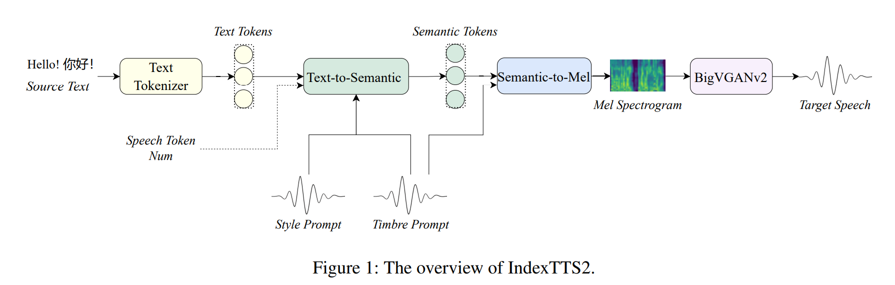
- 主要由三部分组成:
Text-to-Semantic(T2S):- 输入:
- 文本(待合成的文字)
Timbre Prompt(说话人参考音频)Style Prompt(情感参考音频)- 可选的
Duration控制(语义token序列长度)
- 输出
- 语义
token(semantic tokens)
- 语义
- 输入:
Semantic-to-Mel(S2M):一个基于flow-matching的非自回归模型- 输入:
- 语义
token(semantic tokens) - 说话人提示 (音色,
timbre prompt)
- 语义
- 输出:
Mel频谱图
- 输入:
Vocoder(BigVGANv2):把Mel频谱解码成最终的音频波形
2. Text-to-Semantic 详解
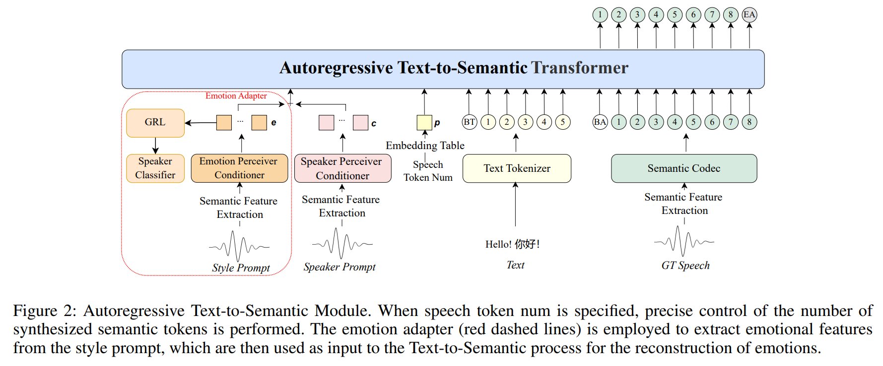
- 这个模块是模型的核心,采用自回归的
Transformer架构,负责将文本和其他条件信息转换为中间的语义表征(Semantic Tokens)。 - 输入:
- 文本序列 (
Text): 经过分词器处理后的文本嵌入 - 说话人音色提示 (
Timbre Prompt): 一段音频,通过预训练的 Speaker Perceiver Conditioner 提取为说话人特征向量 。 - 情感风格提示 (
Style Prompt): 一段音频,通过Emotion Perceiver Conditioner提取为情感嵌入 。 - 时长控制信号 (
Speech Token Num): 一个可选的数字,指定希望生成的语义令牌数量,被转换为时长嵌入 。如果不指定,则用于自由生成。
- 文本序列 (
- 输出:
- 语义令牌序列 (
Semantic Tokens): 模型预测出的语义令牌序列。 GPT隐层状态 ():T2S模块最后一个Transformer层的输出,包含了丰富的文本和上下文信息,会作为增强特征送入后续的S2M模块。
- 语义令牌序列 (
- 监督信号:基准语音 (
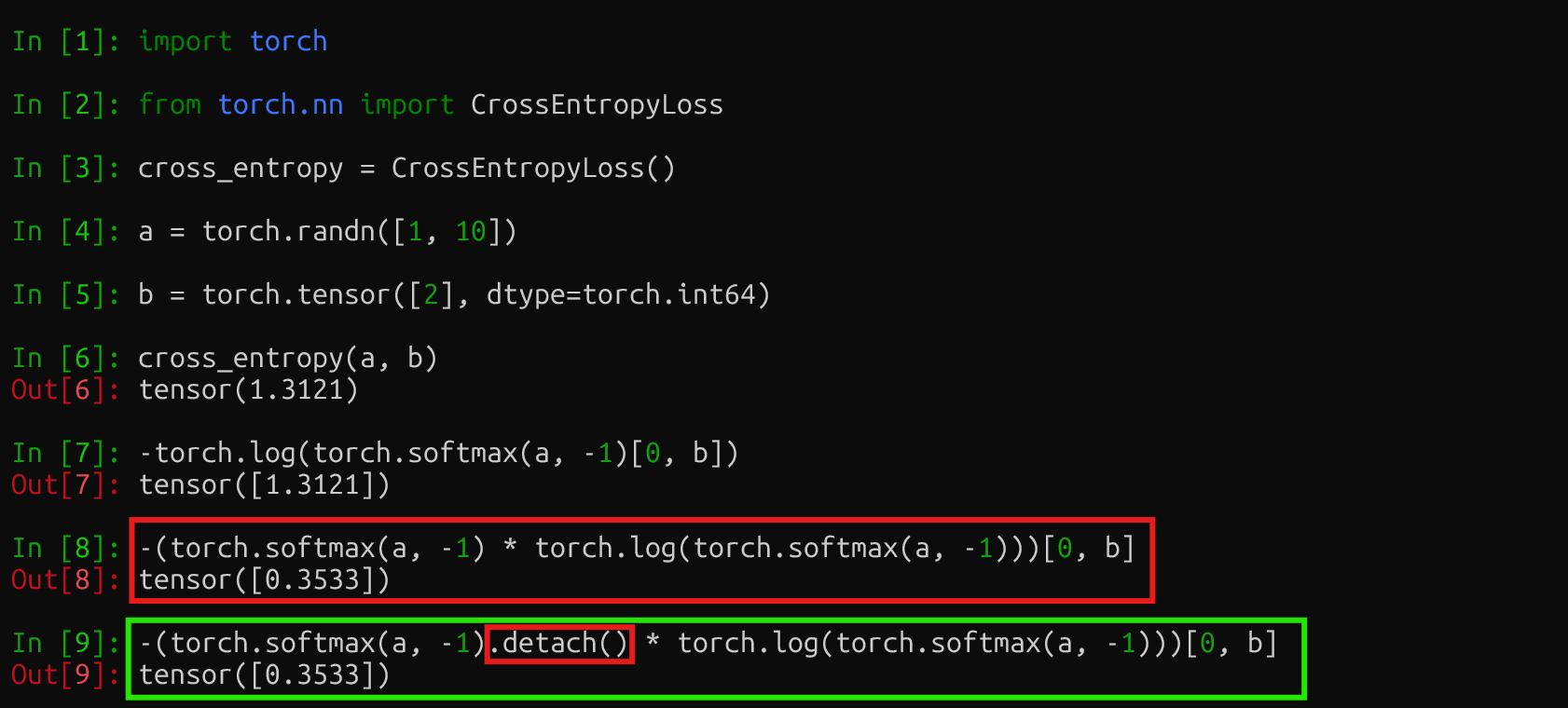
Ground-Truth Speech)。将基准语音通过语义编码器 (Semantic Codec) 转换成真实的语义令牌序列 - 损失函数:交叉熵损失
- 技巧:使用
GRL + speaker classifier,对抗训练,避免style携带timbre信息
3. Semantic-to-Mel 详解
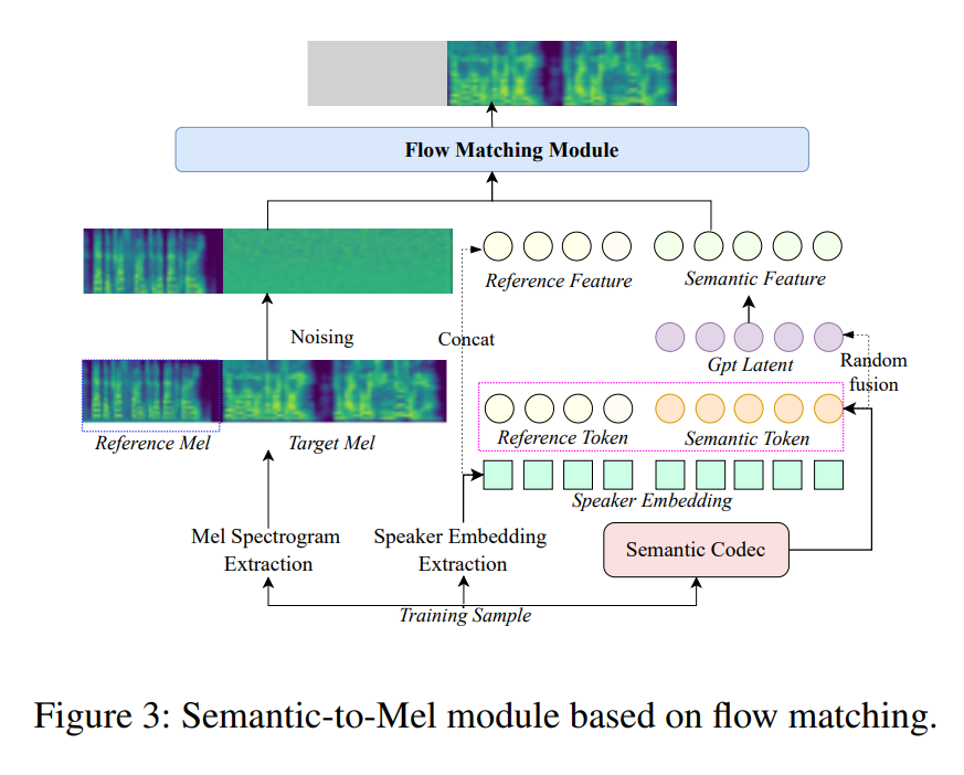
- 该模块基于流匹配 (
Flow Matching) 的非自回归框架,负责将T2S生成的语义令牌序列合成为梅尔频谱图。 - 输入:
- 语义令牌 (): 来自
T2S模块的输出。 GPT隐层状态 (): 来自T2S模块的输出,用于增强语义信息。这两者会通过一个MLP以50%的概率进行随机融合,形成最终的语义表征 。- 说话人嵌入 (
Speaker Embedding): 从音色提示音频中提取的说话人特征,以保证音色的一致性。 - 提示梅尔频谱 (
Prompt Mel-spectrograms): 训练时,输入音频会被随机切分为提示段和目标段,提示段的梅尔频谱作为参考。
- 语义令牌 (): 来自
- 输出:目标梅尔频谱图 (
Target Mel Spectrogram) - 训练方式:模型学习一个常微分方程 (
ODE),将高斯噪声映射到目标梅尔频谱。训练时,目标段的真实梅尔频谱被完全加噪,模型需要学习去噪并重建它。 - 监督信号:目标段的真实梅尔频谱图 ()
- 损失函数:
L1 loss
4. Vocoder 详解
- 输入:
- 由
S2M模块生成的梅尔频谱图 (Mel Spectrogram)。
- 由
- 输出:
- 最终的音频波形 (
Audio Waveform)。
- 最终的音频波形 (
- 直接使用了训练好的
BigVGANv2模型
Thoughts
TTS是个很有趣的领域,直觉上看流媒体平台上有大量的语音数据,应该很容易训练一个TTS模型,但实际上似乎并不是很容易。- 用
GRL来去除style中的timbre信息是个不错的想法。