URL
TL;DR
LLM作为基础预训练模型,由于其参数量极大(以B计)的特点,无法像传统视觉或语言预训练模型一样,在下游任务数据集上全局微调- 本文提出一种非常新颖的
LLM微调方法,不对原始模型参数进行改进,而是在每个任务的Prompt输入之前加入不同长度的虚拟prefix token seqence来实现 - 其中
prefix token seqence实际上是一个 的可学习矩阵- 其中, 表示
prefix token seqence的长度 - 表示原始模型的词嵌入的长度
- 虚拟
token的含义是不是真正来自词表的token,而是无意义的可学习的连续的任务相关的token表征 - 不同任务的可学习矩阵不共享
- 其中, 表示
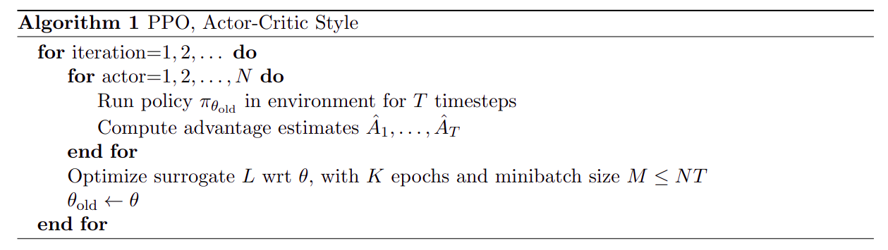
Algorithm
传统 fine tuning 和 prefix tuning 的对比
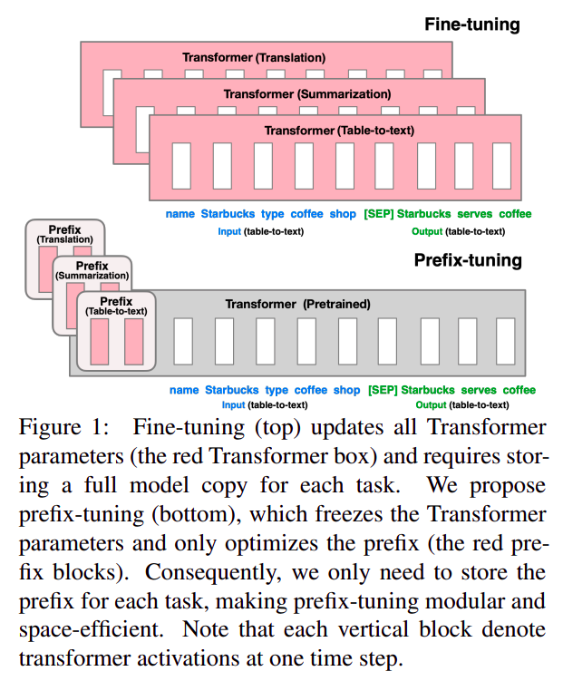
- 传统
fine tuning更新全部模型参数 prefix tuning不更新任何模型参数,只是额外加入了部分参数(虚拟token表征参数)
任务相关应该怎么理解?
- 任务相关是指,每一个任务都需要独立的无法共享的
prefix token表征,而且表征的长度可能不同 - 例如,用预训练的
GPT-2 small+prefix tuning,使其可以做内容总结任务,就需要初始化一个 的矩阵,然后通过有监督训练优化这个虚拟embedding层相关的参数- 其中:
200是通过实验发现的最合适的总结任务prefix token sequence长度 768是GPT-2 small模型真实token embedding的维度
- 其中:
- 如果想用预训练的
GPT-2 small+prefix tuning,使其可以做表格转文本的任务,就需要重新初始化虚拟token embedding矩阵,重新训练
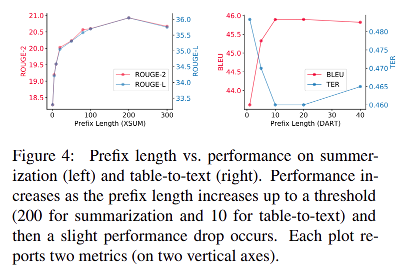
实验证明,对于总结任务,
200是个合适的prefix token sequence长度,对于表格转文本,10长度更合适
prefix tuning 如何适配不同架构的预训练模型?
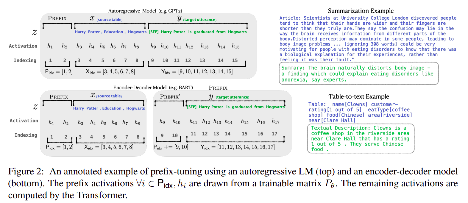
- 对于
GPT系列的Casual Decoder架构,只需要在输入文本token sequence之前加入prefix token sequence - 对于
Encoder Decoder架构,需要在encoder和decoder输入之前都加入prefix,encoder和decoder的prefix token表征可以共享,也可以不共享,具体看任务效果
和 fine tuning 相比,效果如何?
- 在数据充足且任务难度不大的情况下,
prefix tuning效果不差于fine tuning - 由于
prefix没有修改模型原始参数,所以不容易出现full fine tuning中常出现的模型退化问题
Thought
prefix tuning看起来是非常有希望的topic,prompt engineering可挖掘的空间还很大- 这种微调方式实际上还需要存储大模型的所有参数和推理的中间结果用于梯度回传,所以实际微调代价不如想象中小