URL
- paper: https://arxiv.org/pdf/2210.15191
- code: https://github.com/john-hewitt/truncation-sampling/blob/main/src/TruncationVisualization.ipynb
TL;DR
- 常用的
top-p random sampling decoding method可能会导致输出的长文本质量较差 - 本文设计了一种基于熵的动态概率阈值优化
top-p随机采样算法,叫做
Algorithm
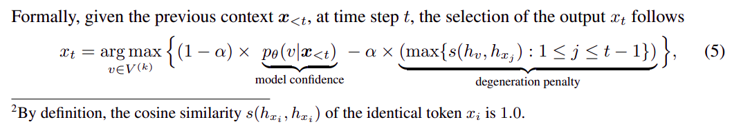
公式表示
其中第一行公式表示随机采样概率值截断到
第二行中 是超参数,通常 ,h 表示输出的熵,,p 表示概率
代码表示
1 | class EtaWarper(transformers.LogitsWarper): |
Thought
- 是
top-p的小升级,计算量较小,算是一个小trick